Building distributed systems means passing messages between devices over a network connection. My research specifically considers networks that have extremely variable latencies or that can be partition prone. This led me to the natural question, “how variable are real world networks?” In order to get real numbers, I built a simple echo protocol using Go and gRPC called Orca.
I ran Orca for a few days and got some latency measurements as I traveled around with my laptop. Orca does a lot of work, including GeoIP look ups, IP address resolution, and database queries and storage. This post, however, is not about Orca. The latencies I was getting were very high relative to the round-trip latencies reported by the simple ping command that implements the ICMP protocol.
At first, I attributed this difference to the database overhead, but it was still far too high. In order to measure the difference between ping and the echo protocol I implemented, I created a branch that strips everything except the communications protocol: a protocol buffers service implemented with gRPC. I believe there are two potential places that introduce the overhead, either in the gRPC communications protocol or in Go itself, for example the garbage collector.
Experiment
To see how much of a difference there is in the overhead of the Go implementation, I simultaneously ran both ping and orca from my house to a server at the University for an hour. I collected slightly under 3600 round-trip latencies (RTTs) for each (there were a few dropped packets). The result was that, on average, ping is approximately 16.384 ms faster than the gRPC protocol, and less variable by 4.933 ms! The variability might be explained by language-specific elements like garbage collection and threading,
but the ease of use of protocol buffers comes at a cost!
The results of the two pings are as follows:
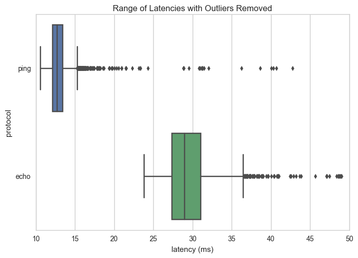
This above figure shows a box plot of the dataset with outliers trimmed using the z-score method and 2 passes. The ends of the bar represent the 5th and 95th percentile respectively, and data points outside the 95th percentile are plotted individually. The box goes from the first to the third quartile and the middle line is the median. As you can see from this plot, there is no overlap from the high percentile of the ping protocol to the lower percentile of the echo protocol. Moreover, the majority of the ping points are in a much smaller range than the majority of the echo protocol points.
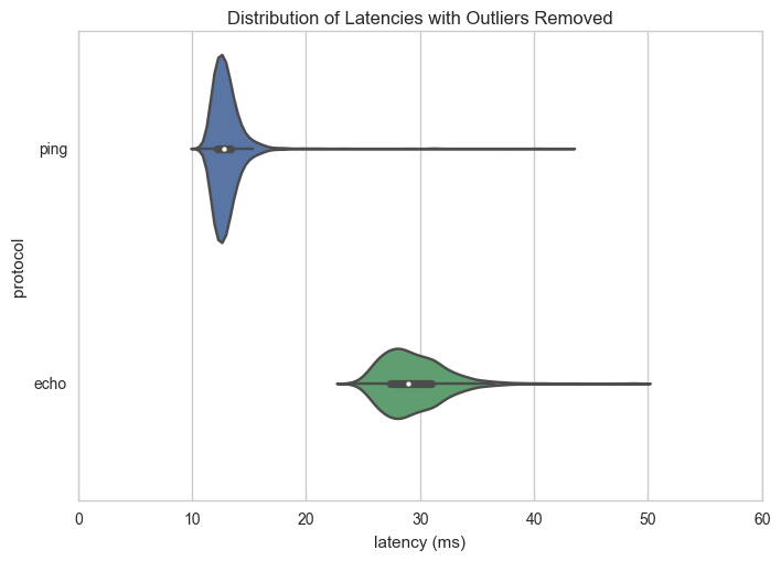
This second image shows the violin plot - such that the curve represents the kernel density estimate (KDE) of the histogram of the data. It then similarly shows the median and the first and third quartiles inside of the violin. Both distributions are significantly right skewed, but the ping distribution has a much steeper curve than the more variable echo protocol.
Here are the raw statistics for the small experiment:
|——-|———–|———–|
| ping | echo | |
|---|---|---|
| count | 3,567 | 3,538 |
| mean | 13.037 ms | 29.431 ms |
| std | 1.877 ms | 2.908 ms |
| min | 10.616 ms | 23.806 ms |
| 25% | 12.169 ms | 27.366 ms |
| 50% | 12.747 ms | 28.989 ms |
| 75% | 13.422 ms | 31.016 ms |
| max | 42.806 ms | 49.039 ms |
| :—— | ———– | ———– |
So what does this mean? Of course, I could do extensive experimentation, moving the laptop and getting different times of day for latency measurements. However, I honestly believe that the one hour test was enough to demonstrate how significant a gap there is between the ping implementation and a gRPC implementation of the communications. In normal systems there will always be some message processing overhead and database accesses, however right off the bat you do incur a significant overhead.
Method
To run the experiment to collect data for comparison (and as documentation in case I have to do this again), I did it as follows. First clone the orca repository:
$ go get github.com/bbengfort/orca/...
You’ll then have to cd into that directory, which is in your $GOHOME/src location. Checkout the ping branch as follows:
$ git fetch
$ git checkout ping
You should see a pretty significant change in the amount of code and the README should indicate you’re in the ping branch. Set up a server to listen for the ping requests:
$ go run cmd/orca listen
If you want, you can run it in silent mode with the -s flag to further reduce latency as much as possible. In silent mode, the command prints nothing to the console. Then run 3600 pings on a different machine as follows:
$ go run cmd/orca -n 3600 ping 1.2.3.4:3265
Make sure you insert the correct IP address and port! As quickly as you can, also start the ping service:
$ ping -c 3600 1.2.3.4
After about an hour, the dataset is sitting at your disposal ready to copy and paste into a text file. You can use the ping_vs_echo.ipynb Jupyter Notebook to perform the analysis. It includes regular expressions to parse each type of line output and to aggregate them into the visualizations you saw above.
Local Subnet
There are many reasons that ping could be faster than gRPC, not just the overhead of serializing and deserializing protocol buffers and HTTP transport. For example, ICMP could be given special routing, ICMP is handled closer to the kernel level, or the fact that ICMP frames are much, much smaller. In order to test this I ran the test from two machines on the same subnet; the violin plot for the distribution is below:
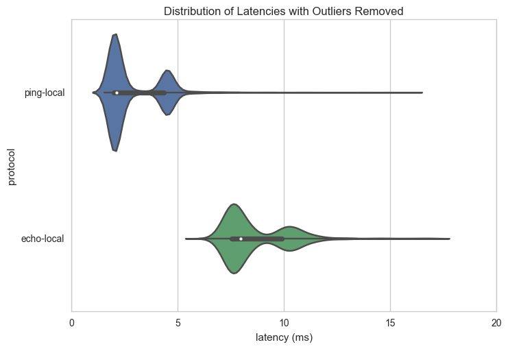
Both ping and echo latencies are much smaller, by approximately the same amount. Because the gap between them is approximately the same percentage (though not fixed), I think this graph identifies clearly what is overhead and what is network latency. However, because the gap is also smaller, it shows that bandwidth and other message traffic may be having an influence in the disparity as well (e.g. that ping has preferential routes through wide area networks).