One of the challenges we’ve been dealing with in the Yellowbrick library is the proper resolution of colors, a problem that seems to have parallels in matplotlib as well. The issue is that colors can be described by the user in a variety of ways, then that description has to be parsed and rendered as specific colors. To name a few color specifications that exist in matplotlib:
- None: choose a reasonable default color
- The name of the color, e.g.
"b"or"blue" - The hex code of the color e.g.
"#377eb8" - The RGB or RGBA tuples of the color, e.g.
(0.0078, 0.4470, 0.6353) - A greyscale intensity string, e.g.
"0.76".
The pyplot api documentation sums it up as follows:
In addition, you can specify colors in many weird and wonderful ways, including full names (‘green’), hex strings (’#008000’), RGB or RGBA tuples ((0,1,0,1)) or grayscale intensities as a string (‘0.8’). Of these, the string specifications can be used in place of a fmt group, but the tuple forms can be used only as kwargs.
Things get even weirder and slightly less wonderful when you need to specify multiple colors. To name a few methods:
- A list of colors whose elements are one of the above color representations.
- The name of a color map object, e.g.
"viridis" - A color cycle object (e.g. a fixed length group of colors that repeats)
Matplotlib Colormap objects resolve scalar values to RGBA mappings and are typically used by name via the matplotlib.cm.get_cmap function. They come in three varieties: Sequential, Diverging, and Qualitative. Sequential and Diverging color maps are used to indicate continuous, ordered data by changing the saturation or hue in incremental steps. Qualitative colormaps are used when no ordering or relationship is required such as in categorical data values.
Trying to generalize this across methodologies is downright difficult. So instead let’s look at a specific problem. Given a dataset, X, whose shape is (n,d) where n is the number of points and d is the number of dimensions, and a target vector, y, create a figure that shows the distribution or relationship of points defined by X, differentiated by their target y. If d is 1 then we can use a histogram, if d is 2 or 3 we can use a scatter plot, and if d >= 3, then we need RadViz or Parallel Coordinates. If y is discrete, e.g. classes then we need a color map whose length is the number of classes, probably a qualitative colormap. If y is continuous, then we need to perform binning or assign values according to a sequential or diverging color map.
So, problem number one is detecting if y is discrete or continuous. There is no automatic way of determining this, so besides having the user directly specify the behavior, I have instead created the following rule-based functions:
def is_discrete(vec):
    """
    Returns True if the given vector contains categorical values.
    """

    # Convert the vector to an numpy array if it isn't already.
    vec = np.array(vec)

    if vec.ndim != 1:
        raise ValueError("can only handle 1-dimensional vectors")

    # Check the array dtype
    if vec.dtype.kind in {'b', 'S', 'U'}:
        return True

    if vec.dtype.kind in {'f', 'c'}:
        return False

    # For vectors of >= than 50 elements
    if vec.shape[0] >= 50:
        if np.unique(vec).shape[0] <= 20:
            return True
        return False

    # For vectors of < than 50 elements
    else:
        elems = Counter(vec)
        if len(elems.keys()) <= 20 and all([c > 1 for c in elems.values()]):
            return True
        return False

    # Raise exception if we've made it to this point.
    raise ValueError(
        "could not determine if vector is discrete or continuous"
    )


def is_continuous(vec):
    """
    Returns True if the given vector contains continuous values. To
    keep things simple, this is currently implemented as not
    is_discrete().
    """
    return not is_discrete(vec)
The rules for determining discrete/categorical values are as follows:
- If it is a string type - True
- If it’s a bool type - True
- If it is a floating point type - False
- If > 50 samples then if there are 20 or fewer discrete values
- If < 50 samples, then if there are 20 or fewer discrete samples that are represented more than once each.
These rules are arbitrary but work on the following test cases:
datasets = (
    np.random.normal(10, 1, 100),   # Normally distributed floats
    np.random.randint(0, 100, 100), # Random integers
    np.random.uniform(0, 1, 1000),  # Small uniform numbers
    np.random.randint(0, 1, 100),   # Binary data (0 and 1)
    np.random.randint(1, 4, 100),   # Three integer clases (1, 2, 3)
    np.random.choice(list('ABC'), 100),   # String classes
)

for d in datasets:
    print(is_discrete(d))
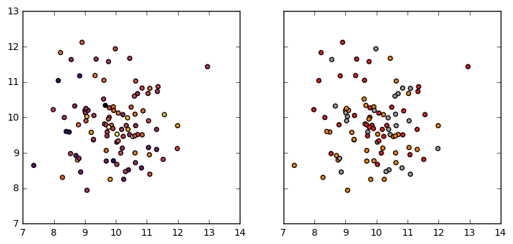
The next step is to determine how best to assign colors for continuous vs. discrete values. One typical use case is to directly assign color values using the target variable, then provide a colormap for color assignment as shown:
# Create some data sets.
X  = np.random.normal(10, 1, (100, 2))
yc = np.random.normal(10, 1, 100)
yd = np.random.randint(1, 4, 100)
f, (ax1, ax2) = plt.subplots(1, 2, sharey=True, figsize=(9,4))

# Plot the Continuous Target
ax1.scatter(X[:,0], X[:,1], c=yc, cmap='inferno')

# Plot the Discrete Target
ax2.scatter(X[:,0], X[:,1], c=yd, cmap='Set1')
Alternatively, the colors can be directly assigned by creating a list of colors. This brings us to our larger problem - how do we create a list of colors in a meaningful way to assign our colormap appropriately? One solution is to use the matplotlib.colors.ListedColormap object which takes a list of colors and can convert a dataset to that list as follows:
- If the input data is in (0,1) - then uses a percentage to assign the color
- If the input data is an integer, then uses it as an index to fetch the color
This means that some work has to be done ahead of time, e.g. discretizing the values or normalizing them.
f, (ax1, ax2) = plt.subplots(1, 2, sharey=True, figsize=(9,4))

# Plot the Continuous Target
norm = col.Normalize(vmin=yc.min(), vmax=yc.max())
cmap = col.ListedColormap([
    "#ffffcc", "#ffeda0", "#fed976", "#feb24c", "#fd8d3c",
    "#fc4e2a", "#e31a1c", "#bd0026", "#800026"
])
ax1.scatter(X[:,0], X[:,1], c=cmap(norm(yc)))

# Plot the Discrete Target
cmap = col.ListedColormap([
    "#34495e", "#2ecc71", "#e74c3c", "#9b59b6", "#f4d03f", "#3498db"
])
ax2.scatter(X[:,0], X[:,1], c=cmap(yd), cmap='Set1')
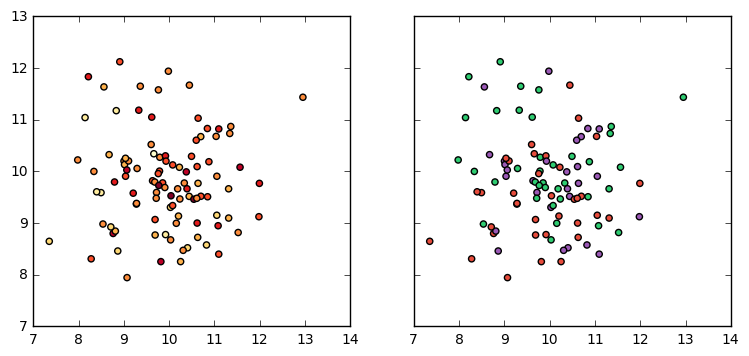
Note that in the above function, the indices 1-3 are used (not the 0 index) since the classes were 1-ordered.
Clearly color handling is tricky, but hopefully these notes will provide us with a reference when we need to continue to resolve these issues developing yellowbrick.