Part of my research is taking me down a path where I want to measure the number of reads and writes from a client to a storage server. A key metric that we’re looking for is throughput — the number of accesses per second that a system supports. As I discovered in a very simple test to get some baseline metrics, even this simple metric can have some interesting complications.
So let’s start with the model. Consider a single server that maintains an in-memory key/value store. Clients can Get (read) values for a particular key and Put (write) values associated with a single key. Every Put creates a version associated with the value that orders the writes as they come in. This model has implications for consistency, even though there is a single server, and we’ll get into that later.
The server handles multiple clients concurrently, each client in its own goroutine. In order to maintain thread safety, a Put request must lock the store while it’s modifying it, ensuring that the value is correctly ordered and not corrupted. On the other hand, a Get request requires only a read lock; multiple goroutines can have a read lock but wait for a write lock to finish. The way the locks work can also inform consistency.
The server and client command line apps are implemented and can be found at github.com/bbengfort/honu.
Throughput is measured by pushing the server to a steady-state of requests. Each client issues a Put request to the server, measuring how long it takes to get a response. As soon as the Put request returns, the client immediately sends another request, and continues to do so for some predetermined amount of time. As the number of clients increases, the server reaches a maximum capacity of requests it can handle in a second, and that is the maximum throughput.
In the first round of experiments, each client is writing to its own key, meaning that there is no conflict on the server end. I utilized the Horvitz Research Cluster to create 25 clients and a single server with low latency connections. Each client runs for 30 seconds sending as many messages sequentially as it possibly can. The throughput is measured as the number of messages divided by the latency of the RPC (and does not include the latency of creating or handling messages at the client end).
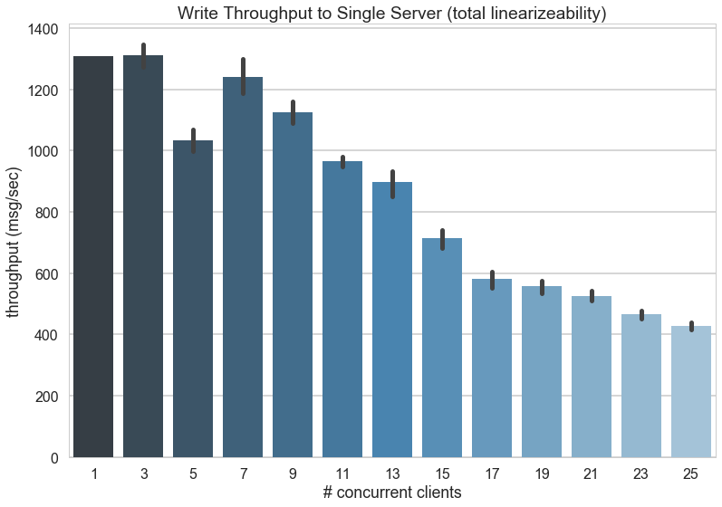
The first results, displayed in the figure above, show the average client throughput as the number of clients increases. This graph met my expectations, in that as the number of clients increases, the throughput goes down. However, when I showed this graph to my advisor, his first response was that it was off in two ways:
- A server should be able to handle far more than 1200 messages per second, probably closer to 10,000 messages per second.
- The throughput should actually increase as the number of clients goes up because the server spends most of its time waiting.
To the first point, I noted that the server was on a VM, potentially the resource scheduling at the hypervisor layer was causing the throughput to be artificially less than a typical server environment. To test this, I ran a client and server as separate processes on the same machine, connecting over the local loopback address to minimize the noise of network constraints. I then compared the VM (bbc29) to a box in my office (lagoon).
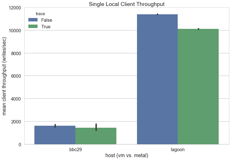
Clearly my advisor was right on the money. On the hardware, the application (with the exact same configuration) performs slightly under 10x better than on the virtual machine. I also tested to see if trace messages (print statements that log connections) affected performance, and they do (blue is without trace, green is with trace) — but not to the amount that can be reconciled with the difference between virtual and hardware performance.
This was a surprise, and made me question whether or not I should rethink using virtual machines in the cloud. However, it was pointed out to me that cloud services do their best not to oversubscribe their hardware, and in an academic setting that may not be the case.
To the second point, the first graph is actually measuring latency at the client, not at the server. So although the server is actually sitting around with spare capacity when there are fewer clients, the throughput can only go as fast as the client does. I think the first graph does show that until about 9 clients or so the performance is plateaued, meaning that the server has capacity to handle all clients at their particular rates. After 9 clients, however, the server is no longer primarily waiting for requests, but is constantly handling requests, and the locks become a factor.

In order to explore this, I instead measured throughput at the server-side. The server records the timestamp of the first message it receives, then maintains the timestamp of the last message it receives, counting the number of messages. It then divides the number of messages by the delta of the last message to the first. The graph above shows the measurements back in the virtual machine cluster of the server-side throughput. This graph is the familiar one, the one it’s “supposed to be” — as the number of clients increases, the throughput increases linearly, until about 9 clients or so when the capacity plateaus at around 16,000 writes per second.
Latency variability, message ordering, and other factors can come into play in a geographic environment — and it is certainly my intention to explore those factors in detail. However, I think it was an important systems lesson to learn the expected shape of baseline environments, so that I will be able to immediately compare graphs I’m getting with the expected form.